Overview
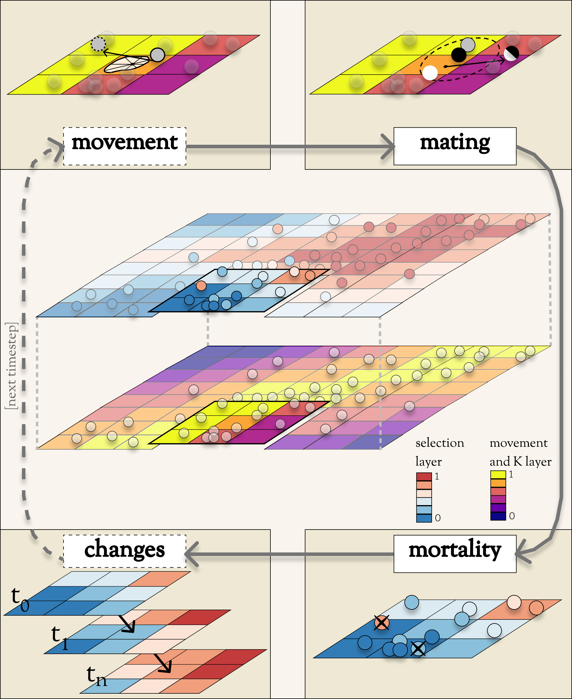
As you’re reading, you may want to refer to the Conceptual Diagram as a useful reference. The primary data structures are depicted in the central image. Most of the key operations are depicted in the cycle of four corner boxes.
Data structures
The following sections discuss the structure and function of the key Geonomics classes. Users will interface with these classes more or less directly when running Geonomics models, so a fundamental understanding of how they’re organized and how they work will be useful.
Landscape and Layer objects
One of the core components of a Geonomics model is the land. The land is
modeled by the Landscape class. This class is an
integer-keyed dict composed of numerous instances of the
class Layer. Each Layer represents a separate
environmental variable (or ‘layer’, in GIS terminology),
which is modeled a 2d Numpy array (or raster; in
attribute ‘rast’), of identical dimensions to each
other Layer in the Landscape
object, and with the values of its environmental variable ‘e’ constrained to
the interval [0 <= e <= 1]. Each Layer can be initialized from its own
parameters subsection within the ‘land’ parameters section of a Geonomics
parameters file.
For each Species
(see Individual, Species, and Community objects, below),
the different Layer layers in the Landscape can be used to model habitat
viability, habitat connectivity, or variables imposing spatially varying
natural selection. Landscape and Layer objects
also contain some metatdata (as public attributes), including
the resolution (attribute ‘res’), upper-left corner (‘ulc’),
and projection (‘prj’), which default to 1, (0,0), and None but
will be set otherwise if some or all of the Layer layers are read in from
real-world GIS rasters.
Genomes, GenomicArchitecture, and Trait objects
Individual objects
(see Individual, Species, and Community objects, below)
can optionally be assigned genomes.
If they are, each Individual’s genome is conceptually modeled as a
L-by-1 array (where L is the genome length,
and 2 is the ploidy, currently fixed at
diploidy) containing 0s and 1s (because
Geonomics strictly models biallelic SNPs, i.e SNPs with ‘0’- and ‘1’-alleles).
(In actuality, the way in which Geonomics stores genomes
depends on the parameter use_tskit.
If use_tskit is True, Geonomics stores genomes by combining
Numpy arrays for non-neutral genotypes with a tskit TableCollection
for neutral genotypes and for the current population’s spatial pedigree.
Although this makes for more complicated data structures,
it optimizes information retention while minimizing memory usage,
keeping Geonomics fast yet nonetheless enabling powerful
spatiotemporal population genomics research.
See tskit.tables.TableCollection, below, for details.
If use_tskit is False, each Individual stores its full genome,
including neutral and non-neutral loci,
as an L-by-2 array, and no special data structures are used.
The choice of whether or not to use tskit depends on the parameterization
of a user’s model, with models requiring larger numbers of independent loci
running more smoothly without tskit.
See the use_tskit section of the Parameters section
for more details.)
The parameter L, as well as numerous other genomic parameters (including
locus-wise starting frequencies of the 1 alleles; locus-wise dominance effects;
locus-wise recombination rates; and genome-wide mutation rates for neutral,
globally deleterious, and adaptive loci), are controlled by the
GenomicArchitecture object pertaining to the Species to which an
Individual belongs. (For the full and detailed list of attributes in a
GenomicArchitecture object, see its class documentation, below.)
The genomes of the initial Individuals
in a simulation are drawn, and those of
Individuals in subsequent generations are recombined (and optionally
mutated) according to the values stipulated
by the GenomicArchitecture of
their Species. The user can create a species with a
GenomicArchitecture and with corresponding
genomes by including a ‘genome’ subsection in that
species’ section of the Geonomics parameters file (and
setting the section’s various parameters to their desired values).
Geonomics can model Individuals’ phenotypes.
It does this by allowing the
user to create an arbitrary number of distinct Traits
for each Species. Each trait is
represented by a Trait object, which
maps genomic loci onto that trait, maps effect sizes (‘alpha’) onto those loci,
and sets the trait’s polygenic selection
coefficient (‘phi’). An Individual’s
phenotype for a given trait is calculated as the ‘null phenotype’ plus a
weighted sum of the products of its ‘effective genotypes’ at all loci
underlying that Trait and the effect sizes (i.e. ‘alpha’) of those loci:
where \(z_{i,t}\) is the phenotype of Individual i for trait t,
\(g_{i, l}\) is the effective genotype of Individual \(i\)
at locus \(l\), and
\(\alpha_{t,l}\) is the effect size of locus \(l\) for trait \(t\).
The ‘null phenotype’ represents the phenotypic value for
an Individual who is homozygyous for
the 0 allele at all loci for a trait.
For monogenic traits the null phenotype is 0 and the effect size is fixed at
0.5 (such that individuals can have phenotypes of 0, 0.5, or 1);
for polygenic traits the null phenotype is 0.5 and effect sizes can be fixed
at or distributed around a mean value (which is controlled in the
parameters file).
The ‘effective genotype’ refers to how the genotype is calculated based on the dominance at a locus, as indicated by the following table of genotypes:
Biallelic genotype |
Codominant |
Dominant |
|---|---|---|
0 : 0 |
0 |
0 |
0 : 1 |
0.5 |
1 |
1 : 1 |
1 |
1 |
(For the full and detailed list of attributes in a Trait object,
see its class documentation, below.)
Note that for maximal control over the GenomicArchitecture
of a Species, the user can set the value of the ‘gen_arch_file’
parameter in the parameters file to the name of a separate CSV file
stipulating the locus numbers, starting 1-allele frequencies, dominance
effects, traits, and inter-locus recombination rates (as columns) of
all loci (rows) in the GenomicArchitecture;
these values will override any other values provided in the ‘genome’
subsection of the species’ parameters.
Individual, Species, and Community objects
Being that Geonomics is an individual-based model, individuals serve as
the fundamental units (or agents) of all simulations. They are represented by
objects of the Individual class.
Each Individual has an index (saved
as attribute ‘idx’), a sex (attribute ‘sex’), an age (attribute ‘age’),
an x,y position (in continuous space; attributes ‘x’ and ‘y’), and a
list of environment values (attribute ‘e’), extracted from the
Individual’s current cell on each Layer
of the Landscape on which the Individual lives.
The Species class is an OrderedDict
(defined by the collections
package) containing all Individauls, (with
their ‘idx’ attributes as keys). If a Species
has a GenomicArchitecture then the Individuals
in the Species will also each have genomes (attribute ‘g’),
and the GenomicArchitecture includes Traits
then each individual will also have a list of
phenotype values (one per Trait; attribute ‘z’) and a
single fitness value (attribute ‘fit’). (These attributes all otherwise
default to None.)
Each Species also has a number of other attributes of interest. Some
of these are universal (i.e. they are created regardless of the
parameterization of the Model to which a Species inheres). These
include: the Species’ name (attribute ‘name’); its current density
raster (a Numpy array attribute called ‘N’); and the number of births,
number of deaths, and terminal population size (i.e. total number of
individuals in the Species) of each timestep (which are
list attributes called ‘n_births’, ‘n_deaths’, and ‘Nt’). If the
Species was parameterized with a
GenomicArchitecture then that will
be created as the ‘gen_arch’ attribute (otherwise this attribute will be
None).
All of the Species in a Model
are collected in the Model’s
Community object. The Community class
is simply an integer-keyed dict
of Species. For the time being, the Community object allows a
Geonomics Model to simulate multiple Species simultaneously on
the same Landscape, but otherwise affords no additional functionality
of interest. However, its implementation will facilitate the potential
future development of methods for interaction between Species.
(e.g. to simulate coevolutionary, speciation, or hybridization scenarios).
Model Objects
Objects of the Model class serve as the main interface between the user
and the Geonomics program. (While it is certainly possible for a user
to work directly with the Landscape
and Species or Community objects to
script their own custom models, the typical user should find that the
Model object allows them accomplish their goals with minimal toil.)
The main affordance of a Model object is the Model.run method,
which, as one could guess, will run the Model. The typical workflow
for creating and running a Model object is as follows:
Create a template paramters file containing the desired sections, by calling
gnx.make_parameters_filewith all revelant arguments;Define the scenario to be simulated, by opening and editing that parameters file (and optionally, creating/editing corresponding files, e.g. genomic-architecture CSV files; or raster or numpy-array files to be used as
Layers);Instantiate a
Modelobject from that parameters file, by callingmod = gnx.make_model('/path/to/params_filename.py');Run the
Model, by callingmod.run().
For detailed information on usage of these functions, see their docstrings.
When a Model is run, it will:
Run the burn-in (until the mininmal burn-in length stipulated in the parameters file and the built-in stationarity statistics determine that the burn-in is complete);
Run the main model for the stipulated number of timesteps;
Repeat this for the stipulated number of iterations (retaining or refreshing the first run’s initial
LandscapeandSpeciesobjects as stipulated).
The Model object offers one other method, however, Model.walk,
which allows the user to run a model, in either ‘burn’ or ‘main’ mode,
for an arbitrary number of timesteps within a single iteration (see its
docstring for details). This is particularly useful for running
Geonomics within an interactive Python session. Thus, Model.run is
primarily designed for passively running numerous iterations of a Model,
to generate data for analysis, whereas Model.walk is primarily designed
for the purposes of learning, teaching, or debugging the package, or
developing, exploring, introspecting, or visaulizing particular Models.
Secondary (i.e. private) classes
The typical user will not need to access or interact with the following classes in any way. They will, however, parameterize them in the parameters file by either leaving or altering their default values. Geonomics sets generally sensible default parameter values wherever possible, but for some scenarios they may not be adequate, and for some parameters (e.g. the window-width used by the _DensityGridStack; see below), there is no “one-size-fits-most” option. Thus, it is important that the user have a basic acquaintance with the purpose and operation of these classes.
_ConductanceSurface
The _ConductanceSurface class allows Geonomics
to model a Species’
realistic movement across a spatially varying landscape. It does this by
creating an array of circular probability distributions (i.e. VonMises
distributions), one for each cell on the Landscape, from which
Individuals choose their directions each time they move. To create the
_ConductanceSurface for a Species,
the user must indicate the Layer
that should be used to create it (i.e. the Layer that represents
landscape permeability for that Species).
The _ConductanceSurface’s
distributions can be simple (i.e. unimodal), such that the
maximum value of the distribution at each cell will point toward the
maximum value in the 8-cell neighborhood; this works best for permeability
Layers with shallow, monotonic gradients, because the differences
between permeability values of neighboring cells can be minor (e.g. a
gradient representing the directionality of a prevalent current).
Alternatively, the distributions can be mixture (i.e. multimodal)
distributions, which are weighted sums of 8 unimodal distributions, one
for each neighboring cell, where the weights are the relative cell
permeabilities (i.e. the relative probabilities that an Individual would
move into each of the 8 neighboring cells); this works best for non-monotonic,
complex permeability Layers (e.g. a DEM of a mountainous region that is
used as a permeability Layer).
(The Landscape is surrounded by a margin of 0-permeability
cells before the _ConductanceSurface is calculated, such
that Landscape edges are treated
as barriers to movement.) The class consists
principally of a 3d Numpy array (y by x by z, where y and x (a.k.a i and j,
or latitude and longitude) are the dimensions of the
Landscape and z is the length of the vector of values
used to approximate the distributions in each cell.
_DensityGridStack
The _DensityGridStack class implements an algorithm for rapid estimating
an array of the local density of a Species. The resulting array has a
spatial resolution equivalent to that of the Landscape,
and is used in all density-dependent operations (i.e. for controlling
population dynamics). The density is estimated
using a sliding window approach, with the window-width determining the
neighborhood size of the estimate (thus essentially behaving like a smoothing
parameter on the density raster that is estimated, with larger window widths
producing smoother, more homogeneous rasters). The window width can be
controlled by setting the ‘density_grid_window_width’ parameter in the
‘mortality’ section of the Species parameters, in a parameters file;
however, if the default value (None) is left then the window width will
default to 1/10th of the width of the Landscape.
Note that setting the window width to a value less than ~1/20th of the
Landscape width is likely to result
in dramatic increases in runtime, so this is generally advised against (but
may be necessary, depending on the user’s interests). The following plot
show the estimated density rasters for a 1000x1000-cell Landscape with
a population of 50,000 individuals, using various window widths:

And this plot shows how _DensityGridStack creation
(plot titled ‘making’) and runtime (plot titled ‘calc’)
scale with window-width for that Landscape:

_KDTree
The _KDTree class is just a wrapper around scipy.spatial.cKDTree.
It provides an optimized algorithm (the kd-tree) for finding
neighboring points within a given search radius.
This class is used for all neighbor-searching operations (e.g. mate-search).
tskit.tables.TableCollection
To enable easy recording of the pedigree of a simulated Species,
Geonomics depends on the Python package tskit (software
that originated as improvements made to the data structures
and algorithms used by the popular coalescent simulator msprime).
Geonomics uses the tskit tables API to store the full history of
individuals, genotypes, mating events, and recombinations for
a Species in a TableCollection object.
This data structure is initiated with a random pedigree
that is backwards-time simulated using msprime
and used as a stand-in (viz. meaningless) pedigree
for a Species’ starting population.
It is then updated with each timestep’s forward-time simulation information,
and it is periodically simplified as recommended by the tskit authors
using tskit’s simplification algorithm.
(The simplification interval can be parameterized by the user.)
Because each individual is stored along with its x,y birth location,
a TableCollection thus
contains the full spatial pedigree of a Species’ current population.
Geonomics additionally provides some wrapper functions,
implemented as Species methods,
for converting the TableCollection to a TreeSequence,
and for calculating statistics and creating visualizations from these
two data structures. (For further details regarding tskit,
see the Python package
documentation
and the associated peer-reviewed
paper.)
_RecombinationPaths
The _RecombinationPaths class contains a large (and customizable)
number of bitarrays, each of which indicates the genome-length
diploid chromatid numbers (0 or 1) for a
recombinant gamete produced by an Individual of a given Species
(henceforth referred to as ‘recombination paths’). These recombination
paths are generated using the genome-wide recombination rates specified by
the Species’ GeonomicArchitecture. They are generated during
construction of the Model, then drawn randomly as needed (i.e.
each time an Individual produces a gamete). This provides a
reasonable trade-off between realistic modelling of recombination and runtime.
_LandscapeChanger and _SpeciesChanger
These classes manage all of the landscape changes and demographic changes
that were parameterized for the Landscape and
Species objects to which they inhere.
The functions creating these changes are defined at the outset,
then queued and called at their scheduled timesteps.
_DataCollector and _StatsCollector
These classes manage all of the data and statistics that should be collected
and written to file for the Model object to which they inhere
(as determined by the parameters file used the create the Model).
The types of data to be collected, or statistics to be calculated, as
well as the timesteps at which and methods by which they’re
collected/calculated and determined at the outset, then the
appropriate functions called at the appropriate timesteps.
Operations
The following sections discuss the mechanics of core Geonomics operations.
Movement and Dispersal
Movement is optional, such that turning off movement will allow the user
to simulate sessile organisms (which will reproduce and disperse,
but not move after dispersal; this distinction is of course irrelevant
for a Species with a maximum age of 1). For Species
with movement, Individuals can
move by two distinct mechanisms. Spatially random movement
is the default behavior; in this case, Individuals
move to next locations that are determined by a random distance drawn
from a Wald distribution and a random direction drawn from a uniform
circular (i.e. Von Mises) distribution. As with most distributions used
in Geonomics, the parameters of these distributions have sensible
default values but can be customized in a Model’s parameters file
(see section ‘Parameters’, below).
The alternative movement mechanism that is available is
movement across a permeability surface,
using a _ConductanceSurface object.
To parameterize a _MovemementSurface for a Species, the user
must create a template parameters file that includes the
necessary parameters section for the Species (i.e.
the user must set ‘movement’ to True and ‘movement_surface’ to True
in the Species’ arguments to the gnx.make_parameters_file
function (see the docstring for that function for details and an example).
Individuals move to next locations determined by a random distance drawn
from a Wald distribution and a random direction drawn from the distribution
at the _ConductanceSurface cell in which which the Individuals
are currently located. For details about _ConductanceSurface creation,
see section ‘_ConductanceSurface’ above, or the class’ docstring.
Dispersal is currently implemeneted identically to spatially random movement
(with the caveat that the an offspring’s new location is determined
relative its parents’ midpoint). But the option to use a
_ConductanceSurface for dispersal will be offered soon.
Reproduction
Each timestep, for each Species, potential mating pairs
are chosen from among all pairs of individuals within
a certain distance of each other (i.e. the mating radius,
which is set in the parameters file).
This choice can be made by strict nearest-neighbor mating,
or pairs can be randomly drawn from within the mating radius
using either uniform or inverse-distance weighted probabilities.
These pairs are subsetted if necessary (i.e. if the Species
requires that Individuals be above a certain reproductive age,
or that they be of opposite sexes, in order to mate; these values
can also be changed from their defaults in the parameters file).
Remaining pairs mate probabilistically (according to a Bernoulli
random draw with probability equal to the Species’ birth
rate, which is also set in the parameters file).
Pairs that are chosen to mate will produce a number of new
offspring drawn from a Poisson distribution (with lambda set in the
parameters file). For each offspring, sex is chosen probablistically
(a Bernoulli random draw with probability equal to the Species’
sex ratio), age set to 0, and location chosen by dispersal from
the parents’ midpoint (see section ‘Movement and Dispersal’). For
Species that have genomes, offspring genomes will be a
fusion of two recombinant genomes from each of the two parents (where
each recombinant is indexed out a parent’s genome using a recombination
path; see section ‘_RecombinationPaths’). For Species
with Traits in their
GenomicArchitectures, offspring phenotypes are
determined at birth. Mutations are also drawn and introduced at this
point (see section ‘Mutation for details).
Mortality
Mortality can occur as a combination of two factors: density dependence
and natural selection. Each Individual has a death decision drawn
as a Bernoulli random variable with
\(P(d_{i}) = 1 - P(s_{i_{dens}})P(s_{i_{fit}})\), where \(P(d_{i})\)
is the probability of death of Individual \(i\), and
\(P(s_{i_{dens}})\) and \(P(s_{i_{fit}})\) are the probabilities of
survival of Individual \(i\) given density-dependence and
fitness. The probability of density-dependent death is contingent on an
Individual’s x,y location
(i.e. the cell in which they’re currently located.
And an Individual’s probability of survival due to fitness
is just equal to the product of their absolute fitness (\(\omega\))
for each of the Individual’s \(m\) Traits.
Thus the equation for an Individual’s probability of death becomes:
The following two sections explain in detail the implementation and calculation of the two halves of the right side of this equation.
Density dependence
Density dependence is implemented using a spatialized form of the class
logistic growth equation (\(\frac{\mathrm{d}
N_{x,y}}{\mathrm{d}t}=rN_{x,y}(1-\frac{N_{x,y}}{K_{x,y}})\),
where the x,y subscripts refer to
values for a given cell on the Landscape).
Each Species has a carrying-capacity raster (a 2d Numpy array;
attribute ‘K’), which is defined in the parameters file to be
one of the Layers in the Landscape.
The comparison between this raster and
the population-density raster calculated at each timestep serves as the
basis for the spatialized logistic growth equation, because both
equations can be calculated cell-wise for the entire extent of the
Landscape (using the Species’
intrinsic growth rate, the attribute
‘R’, which is set in the parameters file).
The logistic equation returns an array of instantaneous population growth rates within each cell. We can derive from this the density-dependent probability of death at each cell by subtracting an array of the expected number of births at each cell, then dividing by the array of population density:
The expected number of births at each cell is calculated as a density raster of the number of succesful mating pairs, multiplied by the expected number of births per pair (i.e. the expectation of the Poisson distribution of the number of offspring per mating pair, which is just the distribution’s paramater lambda).
Selection
Selection on a Trait can exhibit three regimes: spatially divergent,
universal, and spatially contingent. Spatially divergent selection
is the default behavior, and the most commonly used; in this form of
selection, an Individual’s fitness depends on the absolute difference
between the Individual’s phenotypic value and the environmental
value of the relevant Layer (i.e. the Layer that represents the
environmental variable acting as the selective force) in the cell where
the Individual is located.
Universal selection (which can be toggled using the ‘univ_adv’
parameter with a Trait’s section in the parameters file) occurs
when a phenotype of 1 is optimal everywhere on the Landscape. In other
words, it represents directional selection on an entire Species,
regardless of Individuals’ spatial contexts. (Note that this can
be thought of as operating the same as spatially divergent selection,
but with the environmental variable driving natural selection being
represented by an array in which all cells are equal to 1.)
Under spatially contingent selection, the selection coefficient of a
Trait varies across space, such that the strength of selection
is environmentally determined in some way. Importantly, this selection regime
is not mutually exclusive with the other two; in other words,
selection on a certain Trait be both spatially contingent
and either spatially divergent or universal. Spatially contingent selection
can be implemented by providing an array of values (equal in dimensions
to the Landscape) to the ‘phi’ value of a
Trait, rather than a scalar
value (which could be done within the parameters file itself, but may be
more easily accomplished as a step between reading in a parameters file and
instantiating a Model object from it). (Note that non-spatailly
cotingent selection could in fact be thought of as a special case of
spatially contingent selection, but where the array of selection-coefficients
has the same value at each cell.)
All possible combinations of the three selection regimes of selection can all
be thought of as special cases of the following equation for the fitness of
Individual \(i\) for Trait \(p\) (\(\\omega_{i,p}\)):
where \(\\phi_{p;x,y}\) is the selection coefficient of trait
\(p\); \(e_{p;x,y}\) is the environmental variable of the
relevant Layer at Individual \(i\)’s x,y location
(which can also be thought of as the Individual’s optimal
phenotype); \(z_{i;p}\) is Individual \(i\)’s (actual)
phenotype for Trait \(p\); and \(gamma_{p}\) controls
the curvature of the fitness function (i.e. how fitness decreases as
the absolute difference between an Individual’s
optimal and actual phenotypes increases; the default value of 1 causes
fitness to decrease linearly around the optimal phenotypic value).
Importantly, most individuals will experience selection on a given trait that is only a fraction of the strength dictated by a trait’s selection coefficient ($phi_{p;x,y}$). This is because an individual’s fitness for a given trait is determined by the product of the trait’s selection coefficient and the individual’s degree of mismatch to its local environment, ($mid e_{p;x,y} - z_{i;p} mid$ in the previous equation), such that only individuals who are extremely mismatched (e.g. an individual of phenotype 1 or greater who is located in a 0-valued environmental cell) will experience selection equal to or exceeding $phi_{p;x,y}$. Because of this, selection coefficients that would be considered ‘strong’ in classical, aspatial population genetics models will tend to behave less strongly in Geonomics models.
Mutation
Geonomics can model mutations of three different types: neutral, deleterious, and trait mutations. These terms don’t map precisely onto the traditional population-genetic lingo of “neutral”, “deleterious”, and “beneficial”, but they are more or less analogous:
Neutral mutations are the same conceptually in Geonomics as they are in the field of population genetics in general: They are mutations that have no effect on the fitness of the individuals in which they occur.
Deleterious mutations in Geonomics are also conceptually the same in Geonomics and in population genetics: They negatively impact the fitness of the individuals in which they occur.
Trait mutations are the place where the Geonomics concept and the population-genetic concept diverge: In Geonomics, natural selection acts on the phenotype, not the genotype (although these concepts are identical if a
Traitin monogenic), and it is (by default, but not always; see section ‘Selection’, above) divergent. For this reason it would be a misnomer to call mutations that influence a givenTrait’s phenotypes ‘beneficial’ – even though that term is the closest population-genetic concept to this concept as it is employed in Geonomics – because the same mutant genotype in the sameIndividualcould have opposite effects on thatIndividual’s fitness in different environmental contexts (i.e. it could behave as a beneficial mutation is one region of theLandscapebut as a deleterious mutation in another).
Species interactions
This functionality is not yet included available. But the Community class was created in advance recognition that this functionality could be desirable for future versions (e.g. to simulate coevolutionary, speciation, or hybridization scenarios).
Landscape and Species change
For a given Layer, any number of change events
can be planned.
In the parameters file, for each event, the user stipulates the initial
timestep; the final timestep; the end raster (i.e. the array
of the Layer that will exist after the event is complete, defined using
the end_rast parameter); and the
interval at which intermediate changes will occur. When the Model is
created, the stepped series of intermediate Layers (and
_ConductanceSurface objects,
if the Layer that is changing serves as the basis for a
_ConductanceSurface for any Species) will be
created and queued, so that they will swap out accordingly at the appropriate
timesteps.
For a given Species, any number of demographic change events can
also be planned. In the parameters file, for each event, the user
stipulates the type of the event (‘monotonic’, ‘cyclical’, ‘random’, or
‘custom’) as well as the values of a number of associated
parameters (precisely which parameters depdends on the type of event chosen).
As with Landscape change events, all necessary stepwise changes will be
planned and queued when the Model is created, and will be
executed at the appropriate timesteps.
It is also possible to schedule any number of instantaneous changes
to some of the life-history parameters of a Species (e.g. birth rate;
the lambda parameter of the Poisson distribution determining the number of
offspring of mating events). This functionality is currently minimalistic,
but will be more facilitated in future versions.